Modeling granular media using cellular automata (TIPE)
One-and-a-half-year project in the French preparatory track (MP), known as TIPE (travail d’initiative personnelle encadré), December 2020 – July 2022. The work linked cellular automata (CA) to toy models of granular surfaces: custom local rules on a 2D lattice whose long-time dynamics resemble erosion and craterization, implemented in Golly using hashing techniques and macro-cell ideas so large runs remain tractable. Special thanks to Andrew Trevorrow for his kind explanations at the time.
It was also a nice way to dive into the mathematical theory and look at some results such as universality properties, where many cellular automata can replicate a Turing machine while keeping very simple rules. Cellular automata are computationally interesting in their own right, with their already discretized structure and transitions.
1. Project objectives and overview
Objectives. Build intuition and experiments for how strictly local, deterministic updates can mimic aspects of landscape evolution (selective erosion, defect amplification, heterogeneous strength). Connect practice (rules, simulators, performance) to the classical mathematical characterization of global CA maps.
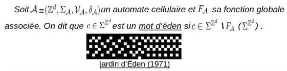
Mathematical definition (cellular automaton). Fix a countable set of cells L (here typically L = ℤd), a finite alphabet S, and a finite neighbourhood N ⊂ L (often invariant under a group action of the translation group, e.g. the von Neumann or Moore neighbourhood in ℤ2). A local rule is a map f : SN → S. A configuration is a map c : L → S. The associated global map F : SL → SL is
F(c)x := f ( (cx+n)n ∈ N ) for all x ∈ L.
Time evolution is the discrete dynamical system ct+1 = F(ct). The full configuration space SL carries the product topology. When S is finite, each factor is compact (discrete finite space), so Tychonoff’s theorem yields compactness of SL.
2. Inspiring examples
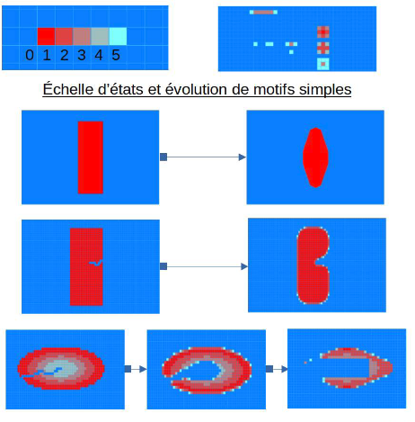
Patterns and “rugs”. Even very simple rules on ℤ2 can produce ordered, almost textile-like motifs (periodic or quasi-periodic colour bands sometimes called Persian rug patterns), coexisting with disordered invasion fronts—useful visual anchors when tuning rules toward textured landforms.
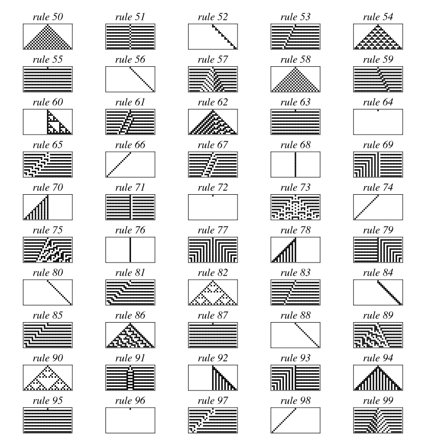
Elementary rules (1D). On ℤ with two states and nearest-neighbour neighbourhood, there are 256 Wolfram elementary rules; their space–time diagrams show how minimal neighbourhoods already generate complexity, chaos, or self-similarity—good sanity checks before designing 2D custom neighbourhoods.
Classic rule families and notation. Many standard rules are specified in compact Birth / Survival form for outer-totalistic life-like automata on ℤ2: Bb1b2… / Ss1s2… lists total neighbour counts that cause a dead cell to become alive (birth) or a live cell to survive. Example: Conway’s Game of Life is B3/S23. The letter N in informal shorthand often refers to the neighbourhood shape (e.g. von Neumann vs Moore) that defines which cells enter the neighbour count. Beyond Life-like rules, well-known landmarks include Langton’s loops (self-reproducing cycles in a CA with many states), Brian’s Brain, and other seminal rule tables (Generations, Larger than Life, …).
3. Simple modeling
HashLife (Bill Gosper, early 1980s) memoises recurring macro-patterns of cells so the simulator can jump in time when the same subpattern reappears—especially effective for Conway’s Life and close variants. See also mafm/HashLife on GitHub for algorithm notes and code. Together with hierarchical macro-cells, this is what makes “absurdly large” universes explorable in practice.
Golly is an open-source CA laboratory: many built-in rules, HashLife-style acceleration where applicable, huge tori or bounded grids, and Python/Lua scripting—ideal for batching custom erosion experiments and checking visual plausibility.
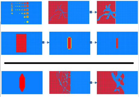
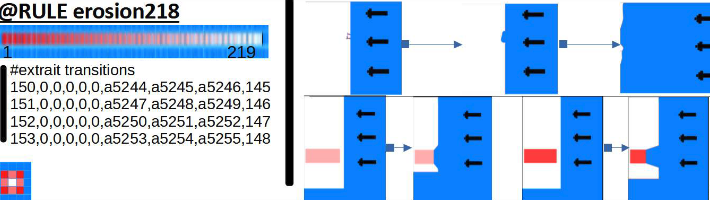
@RULE erosion218). Left: excerpt of encoded transitions; right: simulation panels where interface geometry couples to the rule table—illustrating how different erosion prescriptions change the speed and anisotropy of retreating boundaries.
4. Curtis–Hedlund–Lyndon theorem
We state the theorem on the full shift in dimension d (the same idea extends to any countable group acting by shifts). Write G = ℤd, let S be finite, and let
X = SG = { x : G → S }
equipped with the product topology. For v ∈ G, the shift σv : X → X is (σv(x))g = xg+v. A map F : X → X commutes with the shift action if σv ∘ F = F ∘ σv for all v ∈ G.
Framework. S finite, X compact metrizable, shifts σv homeomorphisms. “Cellular automaton” means: there exist a finite set N ⊂ G and a map f : SN → S such that for every x ∈ X and every g ∈ G,
(F(x))g = f ( (xg+n)n ∈ N ).
Theorem (Curtis–Hedlund–Lyndon). A map F : X → X is the global map of a cellular automaton (i.e. admits some finite N and local rule f as above) if and only if F is continuous (for the product topology) and shift-equivariant (σv ∘ F = F ∘ σv for all v ∈ G).
Definitions used in the proof. A subset U ⊂ X is open if every x ∈ U has a neighbourhood contained in U; it is closed if X \ U is open; it is clopen if it is both open and closed. For a finite window W ⊂ G and a pattern p : W → S, the cylinder set is C(W, p) := { x ∈ X : x|W = p }, where x|W denotes the restriction of the configuration x to coordinates in W.
In the product topology on X = SG (with finite discrete alphabet S), cylinders are basic clopen sets.
Proof
We prove both implications; the easy direction is “local rule ⇒ topology and symmetry”; the converse is the conceptual core of the theorem.
(⇒) If F is a CA global map, then F is continuous and shift-equivariant.
Shift-equivariance. For all x, g, v:
(σv(F(x)))g = (F(x))g+v = f((xg+v+n)n ∈ N) = f((σv(x))g+n)n ∈ N) = (F(σv(x)))g.
Continuity. Fix a coordinate g ∈ G. The map πg ∘ F : X → S depends only on coordinates in the finite set g + N. Hence (πg ∘ F)−1({s}) is a cylinder set (clopen) for each s ∈ S. Finite intersections and unions of cylinders are clopen; since the alphabet is finite, F is continuous when S is given the discrete topology (inverse image of every cylinder in the subbasis of the codomain product topology is clopen). Thus F is continuous on X.
(⇐) If F is continuous and shift-equivariant, then F is a CA global map.
Step 1 — fibre at the origin. Let π0 : X → S be projection to the cell at 0 ∈ G, and consider h := π0 ∘ F : X → S. For each symbol a ∈ S, the singleton {a} is clopen in S, so
Ua := h−1({a}) = { x ∈ X : (F(x))0 = a }
is clopen in X. The family {Ua}a ∈ S is a finite partition of X into disjoint clopens.
Step 2 — clopens are finite unions of cylinders. In the full shift X = SG with S finite, every clopen subset is a finite disjoint union of cylinder sets
C(W, p) := { x ∈ X : x|W = p },
where W ⊂ G is finite and p : W → S. (Idea: clopens are compact-open; cylinder sets form a basis; refine any clopen to a finite disjoint union of basic cylinders.) For each a, write Ua as such a union. Let W0 be the union of all finite windows W that appear in these unions, over all a ∈ S. Then W0 is finite.
Step 3 — (F(x))0 depends only on coordinates in W0. Say that x and y agree on W0 if xw = yw for every w ∈ W0. This is an equivalence relation; each class is a cylinder C(W0, p) for some pattern p. Because each Ua is a disjoint union of cylinders whose coordinate windows lie in W0, every such cylinder C(W0, p) is contained in a unique fibre Ua (the sets Ua partition X). Hence if x and y agree on W0, they lie in the same Ua, so h(x) = h(y), i.e. (F(x))0 = (F(y))0.
Step 4 — propagate to every cell by shift-equivariance. Fix g ∈ G. Using σg ∘ F = F ∘ σg,
(F(x))g = (σg(F(x)))0 = (F(σg(x)))0.
Step 3 applied to σg(x) shows (F(σg(x)))0 depends only on values of σg(x) on W0, i.e. on values of x on g + W0. Therefore (F(x))g depends only on coordinates xg+n with n ∈ W0. Set N := W0 as the neighbourhood of the identity. Then (F(x))g is determined by (xg+n)n ∈ N.
Step 5 — define the local rule. For a pattern p : N → S, choose any configuration x whose restriction to N equals p (arbitrary values elsewhere). Define f(p) := (F(x))0. Step 3 implies (F(x))0 depends only on x on N = W0, so f is well-defined. For any g, Step 4 gives (F(x))g = f((xg+n)n ∈ N). Thus F is a cellular automaton global map. ∎
Remark (where compactness hides). The “hard” direction uses that SG is compact and totally disconnected, so clopen sets are finite unions of cylinders; on non-compact subshifts one must restrict to maps between subshifts satisfying additional closedness hypotheses.